source("00_init.R")
source("02_projection_scores.R")

#knee kinematic data for individuals with PD
PD_data <- readRDS("Datasets/left_knee_data.RDS")

#data on gold-standard outcomes for individuals with PD
PDGinfo <- read_excel("Datasets/PDGinfo.xlsx")

#knee kinematic data for healthy participants
healthy_data <- readRDS("Datasets/healthy_knee_data.RDS")Vignette on MFPCA for Gait data
Preliminaries
We load R libraries, and an R function to compute MFPCA projection scores.
Datasets
We use left knee flexion-extension data from two open source datasets.
Parkinson’s Disease
The first dataset is from individuals living with Parkinson’s Disease. This is obtained from:
Boari, Daniel (2021). A dataset of overground walking full-body kinematics and kinetics in individuals with Parkinson’s disease. figshare. Dataset. https://doi.org/10.6084/m9.figshare.14896881.v4
Healthy Dataset
The second dataset is from healthy individuals. This is obtained from:
Helwig, N. & Hsiao-Wecksler, E. (2016). Multivariate Gait Data. Dataset. UCI Machine Learning Repository. https://doi.org/10.24432/C5861T.
Please see “01_combine_datasets.R” to see how left knee flexion-extension data is extracted from the datasets.
The PD dataset is shown below. Four subjects do not have UPDRS scores recorded, so they are excluded from this analysis.
PD_data <- PD_data %>%
  filter(!(Subject %in% c("SUB04", "SUB23", "SUB25", "SUB26")))

head(PD_data)
Subject Medication Task Joint Type Angle Gait cycle [%] Stride value
1 SUB01 off walk Left Knee Ang 1 4 16.62962
2 SUB01 off walk Left Knee Ang 1 7 17.59559
3 SUB01 off walk Left Knee Ang 1 10 14.71655
4 SUB01 off walk Left Knee Ang 1 13 15.91208
5 SUB01 off walk Left Knee Ang 1 16 18.99039
6 SUB01 off walk Left Knee Ang 1 19 17.14074In addition to kinematic data, we have data on clinical outcomes, which are tidied below.
PDGinfo <- PDGinfo %>%
  filter(!(ID %in% c("SUB04", "SUB23", "SUB25", "SUB26")))

head(PDGinfo)
# A tibble: 6 × 61
ID Gender Age `Height (cm)` `Weight (kg)` `BMI (kg/m2)`
<chr> <chr> <dbl> <dbl> <dbl> <dbl>
1 SUB01 M 58 168 69 24.4
2 SUB02 F 53 170 62.6 21.6
3 SUB03 M 69 165 76.5 28.1
4 SUB05 M 68 169 68.9 24.1
5 SUB06 F 77 152. 60.2 26.2
6 SUB07 F 61 158. 60.5 24.1
# ℹ 55 more variables: `Ortho-Prosthesis` <chr>, `Years of formal study` <dbl>,
# `Disease duration (years)` <dbl>,
# `L-Dopa equivalent units (mg•day-1)` <dbl>, `FoG group` <chr>,
# `FoG-Q (score)` <dbl>, `Initial symptoms` <chr>,
# `Is there a family history of PD? Who?` <chr>,
# `Do you feel improvement after using the antiparkinsonian medicine?` <chr>,
# `Have you ever had any type of surgery? Which?` <chr>, …diagnosis_wide <- data.frame(Subject=PDGinfo$ID,
UPDRS_II_OFF= PDGinfo$`OFF - UPDRS-II`,
UPDRS_III_OFF= PDGinfo$`OFF - UPDRS-III`,
UPDRS_II_ON=PDGinfo$`ON - UPDRS-II`,
UPDRS_III_ON=PDGinfo$`ON - UPDRS-III`)Visualising knee flexion-extention curves
We visualise the kinematic data, focusing on on just four patients. We illustrate the knee flexion-extension curves over the Gait cycle on two occasions per person: when they are on medication, versus when they are off medication.
plot_data <- PD_data %>% filter(Subject %in%
                                   c("SUB01", "SUB02", "SUB03", "SUB07"))

plot_data$Subject <- factor(plot_data$Subject)
levels(plot_data$Subject) =c("Subject 01", "Subject 02", "Subject 03", "Subject 07")

p <- ggplot(plot_data, aes(x=`Gait cycle [%]`, y=value, group=Stride)) +
  geom_line(color="grey30") +
  theme_bw()+
  theme(strip.text.y = element_text(angle = 0), # 0 makes text horizontal
        strip.background = element_rect(fill = "white", color = "black"))+
  facet_grid(Medication~Subject) +
  ylab("Knee flexion-extension angle")

p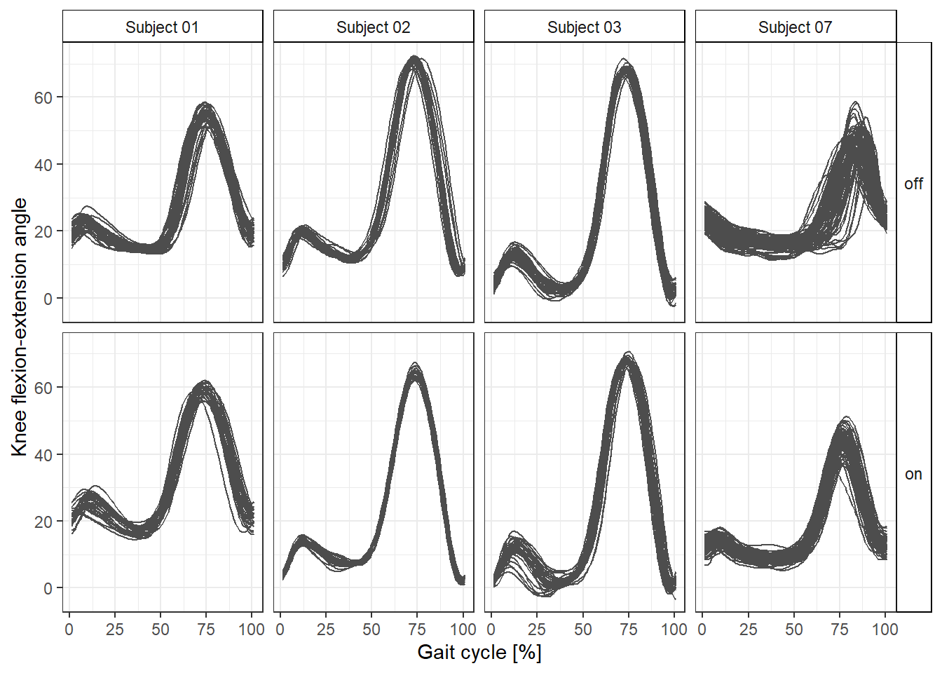
Fitting MFPCA on healthy dataset
We fit MFPCA on healthy dataset. This requires first putting data wide format.
healthy_data <- readRDS("Datasets/healthy_knee_data.RDS")
healthy_wide_dat <- healthy_data %>%
  dplyr::select(Subject, `Gait cycle [%]`, Stride, Angle) %>%
  mutate(Subject_Stride = interaction(Subject, Stride, sep = "_"))

healthy_wide_dat <- healthy_wide_dat %>%
  pivot_wider(id_cols=Subject_Stride,
              names_from=`Gait cycle [%]`,
              values_from=Angle)

healthy_wide_dat <- healthy_wide_dat %>% separate(
  Subject_Stride,
  into = c("Subject", "Stride"),
  sep = "_",
  convert = TRUE
)
We fit MFPCA with the mfpca.face() function in the refund package. We fit 10 principal components.
k=10
increments=1:100

#two-level mfpca
res_healthy_2way <- mfpca.face(Y = as.matrix(healthy_wide_dat[,-c(1:3)]),
                               id=healthy_wide_dat$Subject,
                               npc = c(k,k))

res_healthy_2way_results <- data.frame(Gait=increments,
                                       e1.FPC1=res_healthy_2way$efunctions$level1[,1],
                                       e1.FPC2=res_healthy_2way$efunctions$level1[,2],
                                       e1.FPC3=res_healthy_2way$efunctions$level1[,3],
                                       e2.FPC1=res_healthy_2way$efunctions$level2[,1],
                                       e2.FPC2=res_healthy_2way$efunctions$level2[,2],
                                       e2.FPC3=res_healthy_2way$efunctions$level2[,3])

fpca_results_healthy <- res_healthy_2way_results %>% pivot_longer(cols=-c(Gait), names_to="e", values_to="Eigenfunction")
fpca_results_healthy$Level <- substr(fpca_results_healthy$e, 2, 2)
fpca_results_healthy$Level <- ifelse(fpca_results_healthy$Level==1, "Between-subject", "Within-subject")
fpca_results_healthy$FPC <- substr(fpca_results_healthy$e, 4, 7)

example_dat <- data.frame(Gait=increments,
                          mean= res_healthy_2way$mu,
                          exp1 = res_healthy_2way$mu + 7*res_healthy_2way$efunctions$level1[,1],
                          exp2 = res_healthy_2way$mu + 7*res_healthy_2way$efunctions$level1[,2])


plot_mean <- ggplot(data=example_dat, aes(x=Gait, y=mean)) +geom_line(linewidth=1.1)+
  geom_line(aes(x=Gait, y=exp1), linetype="longdash", col="#3B528B", linewidth=1.1 )+
  geom_line(aes(x=Gait, y=exp2),  linetype="dotdash", col="darkorange", linewidth=1.1)+

  theme_bw()  + ylab("Angle") + ggtitle("(A) Mean Function + Eigenfunctions")

# eigenvalues from mfpca.face
evals1 <- res_healthy_2way$evalues$level1   # between-subject
evals2 <- res_healthy_2way$evalues$level2    # within-subject

# proportion of variance explained
pve1 <- paste0(round(evals1 /sum(evals1)*100, 2), "%")
pve2 <- paste0(round(evals2 / sum(evals2)*100, 2), "%")

var_exp_1 <- data.frame(FPC= paste0("FPC", 1:3), Level="Between-subject", value=pve1[1:3])
var_exp_2 <- data.frame(FPC= paste0("FPC",1:3), Level="Within-subject", value=pve2[1:3])

sum(evals1[1:3])/sum(evals1)
[1] 0.8861358#88.6% of variance explained by the first three eigenfunctions
var_exp <- rbind(var_exp_1, var_exp_2, x=-Inf, y=Inf)
plot_efunction <- ggplot(fpca_results_healthy, aes(x=Gait, y=Eigenfunction)) + geom_line() + theme_bw()+
theme(
strip.text.y = element_text(angle = 0), # 0 makes text horizontal
strip.background = element_rect(fill = "white", color = "black")
) +
geom_text(
data = var_exp %>% filter(FPC %in% c("FPC1", "FPC2", "FPC3", "FPC4")),
aes(x = 89, y = 2, label = value),
inherit.aes = FALSE)+
facet_grid(FPC~Level) + ggtitle("(B) Eigenfunctions")
plot_scores <- ggplot(data = data.frame(score1=res_healthy_2way$scores$level1[,1],
score2=res_healthy_2way$scores$level1[,2]),
aes(x=score1, y=score2)) + theme_bw()+geom_point()+
xlab("Subject-level FPC1 score") + ylab("Subject-level FPC2 score") +
ggtitle("(C) Subject-level scores")
healthy_fpca <- ggarrange(ggarrange(plot_mean, plot_scores, ncol=1),
plot_efunction, widths=c(0.4, 0.6), ncol=2 )
healthy_fpca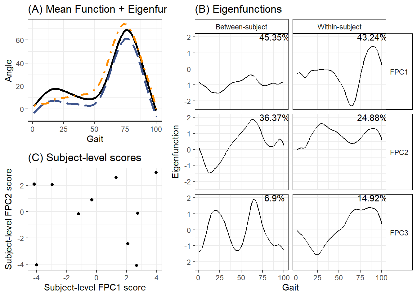
MFPCA projection scores on PD dataset
We first prepare the PD dataset by arranging it in wide format. We also obtain the mean peak of the swing phase as a scalar metric which may be of interest.
wide_dat <- PD_data %>%
dplyr::select(Subject, Medication, `Gait cycle [%]`, Stride, value) %>%   mutate(Subject_Stride = interaction(Subject, Stride, Medication, sep = "_"))

wide_dat <- wide_dat %>%
  pivot_wider(id_cols=Subject_Stride,
              names_from=`Gait cycle [%]`,
              values_from=value)

wide_dat <- wide_dat %>%
  separate(Subject_Stride,
           into = c("Subject", "Stride", "Medication"),
           sep = "_",   convert = TRUE )

#separate data into on and off medication
off_dat <- wide_dat %>% filter(Medication=="off")
on_dat <- wide_dat %>% filter(Medication=="on")


#Obtain Mean peak of swing phase
peak_data <- PD_data %>% group_by(Subject, Medication, Stride) %>%
  summarise(peak=max(value))
peak_data <- peak_data %>% group_by(Subject, Medication) %>%
  summarise(mean_peak=mean(peak))
We now use the pre-prepared functions to obtain projection scores.
#project PD data onto two level mfpca healthy
predicted_scores_off = predict_mfpca_scores_wide(
  res_healthy_2way,
  off_dat[,-c(1:3, 104)],
  off_dat$Subject,
  res_healthy_2way$sigma2)

predicted_scores_off = predicted_scores_off %>%
  dplyr::select(ID, L1_PC1, L1_PC2, L1_PC3) %>%
  distinct()
We regress the MFPCA projection scores against the clinical outcomes (MDS-UPDRS Part II and Part III). We compare these with regression of the mean peak of the swing phase against the clinical outcomes.
pd_dat <- data.frame(FPC1=predicted_scores_off$L1_PC1,
                            FPC2=predicted_scores_off$L1_PC2,
                            FPC3=predicted_scores_off$L1_PC3,
                            UPDRS_II=as.numeric(diagnosis_wide$UPDRS_II_OFF),
                            UPDRS_III=as.numeric(diagnosis_wide$UPDRS_III_OFF),
mean_peak=peak_data[peak_data$Medication=="off", "mean_peak"])

summary(lm(pd_dat$FPC1~pd_dat$UPDRS_II))
Call:
lm(formula = pd_dat$FPC1 ~ pd_dat$UPDRS_II)

Residuals:
    Min      1Q  Median      3Q     Max
-8.2654 -3.9514  0.5861  3.0352  7.2479

Coefficients:
                Estimate Std. Error t value Pr(>|t|)
(Intercept)      1.93773    2.05561   0.943    0.357
pd_dat$UPDRS_II  0.04108    0.26834   0.153    0.880

Residual standard error: 4.715 on 20 degrees of freedom
Multiple R-squared:  0.00117,   Adjusted R-squared:  -0.04877
F-statistic: 0.02343 on 1 and 20 DF,  p-value: 0.8799
p1 <- ggplot(pd_dat, aes(x=UPDRS_II, y=FPC1)) +geom_point() + xlab("")+ylab("FPC1")+theme_bw() +
geom_smooth(method = "lm", se = FALSE, color = "blue") +
annotate(
"text",
x = Inf,
y = Inf,
label ="p ==0.880 * ',' ~ R^2 == 0.001",
parse=TRUE,
hjust = 1.1,
vjust = 1.1
)
summary(lm(pd_dat$FPC2~pd_dat$UPDRS_II))
Call:
lm(formula = pd_dat$FPC2 ~ pd_dat$UPDRS_II)

Residuals:
    Min      1Q  Median      3Q     Max
-5.8152 -1.7597 -0.2274  1.9541  5.5848

Coefficients:
                Estimate Std. Error t value Pr(>|t|)
(Intercept)       3.6280     1.2928   2.806  0.01090 *
pd_dat$UPDRS_II  -0.6021     0.1688  -3.568  0.00193 **
---
Signif. codes:  0 '***' 0.001 '**' 0.01 '*' 0.05 '.' 0.1 ' ' 1

Residual standard error: 2.965 on 20 degrees of freedom
Multiple R-squared:  0.3889,    Adjusted R-squared:  0.3583
F-statistic: 12.73 on 1 and 20 DF,  p-value: 0.001928
p2 <- ggplot(pd_dat, aes(x=UPDRS_II, y=FPC2)) +geom_point() + xlab("")+ylab("FPC2")+ theme_bw() +
geom_smooth(method = "lm", se = FALSE, color = "blue") +
annotate(
"text",
x = Inf,
y = Inf,
label ="p ==0.00193 * ',' ~ R^2 == 0.39",
parse=TRUE,
hjust = 1.1,
vjust = 1.1
)
summary(lm(pd_dat$FPC3~pd_dat$UPDRS_II))
Call:
lm(formula = pd_dat$FPC3 ~ pd_dat$UPDRS_II)

Residuals:
    Min      1Q  Median      3Q     Max
-6.1607 -1.6500  0.2676  1.2447  5.2832

Coefficients:
                Estimate Std. Error t value Pr(>|t|)
(Intercept)       5.0115     1.2012   4.172 0.000470 ***
pd_dat$UPDRS_II  -0.6834     0.1568  -4.359 0.000304 ***
---
Signif. codes:  0 '***' 0.001 '**' 0.01 '*' 0.05 '.' 0.1 ' ' 1

Residual standard error: 2.755 on 20 degrees of freedom
Multiple R-squared:  0.4871,    Adjusted R-squared:  0.4615
F-statistic:    19 on 1 and 20 DF,  p-value: 0.0003043
p3 <- ggplot(pd_dat, aes(x=UPDRS_II, y=FPC3)) +geom_point()+ xlab("") +ylab("FPC3")+ theme_bw() +
geom_smooth(method = "lm", se = FALSE, color = "blue") +
annotate(
"text",
x = Inf,
y = Inf,
label ="p ==0.0003 * ',' ~ R^2 == 0.49",
parse=TRUE,
hjust = 1.1,
vjust = 1.1
)
summary(lm(pd_dat$FPC1~pd_dat$UPDRS_III))
Call:
lm(formula = pd_dat$FPC1 ~ pd_dat$UPDRS_III)

Residuals:
    Min      1Q  Median      3Q     Max
-8.3488 -3.8603  0.5175  3.1408  6.9704

Coefficients:
                  Estimate Std. Error t value Pr(>|t|)
(Intercept)       2.474369   2.475161   1.000    0.329
pd_dat$UPDRS_III -0.009911   0.085494  -0.116    0.909

Residual standard error: 4.716 on 20 degrees of freedom
Multiple R-squared:  0.0006714, Adjusted R-squared:  -0.04929
F-statistic: 0.01344 on 1 and 20 DF,  p-value: 0.9089
p11 <- ggplot(pd_dat, aes(x=UPDRS_III, y=FPC1)) +geom_point()+ xlab("") +ylab("")+theme_bw() +
geom_smooth(method = "lm", se = FALSE, color = "blue") +
annotate(
"text",
x = Inf,
y = Inf,
label ="p ==0.909 * ',' ~ R^2 == 0.001",
parse=TRUE,
hjust = 1.1,
vjust = 1.1
)
summary(lm(pd_dat$FPC2~pd_dat$UPDRS_III))
Call:
lm(formula = pd_dat$FPC2 ~ pd_dat$UPDRS_III)

Residuals:
    Min      1Q  Median      3Q     Max
-7.7635 -1.6725  0.8497  1.8255  5.6590

Coefficients:
                 Estimate Std. Error t value Pr(>|t|)
(Intercept)       3.48564    1.74965   1.992   0.0602 .
pd_dat$UPDRS_III -0.14669    0.06043  -2.427   0.0248 *
---
Signif. codes:  0 '***' 0.001 '**' 0.01 '*' 0.05 '.' 0.1 ' ' 1

Residual standard error: 3.334 on 20 degrees of freedom
Multiple R-squared:  0.2275,    Adjusted R-squared:  0.1889
F-statistic: 5.891 on 1 and 20 DF,  p-value: 0.02479
p22 <- ggplot(pd_dat, aes(x=UPDRS_III, y=FPC2)) +geom_point()+ xlab("") +ylab("")+ theme_bw() +
geom_smooth(method = "lm", se = FALSE, color = "blue") +
annotate(
"text",
x = Inf,
y = Inf,
label ="p ==0.0248 * ',' ~ R^2 == 0.23",
parse=TRUE,
hjust = 1.1,
vjust = 1.1
)
summary(lm(pd_dat$FPC3~pd_dat$UPDRS_III))
Call:
lm(formula = pd_dat$FPC3 ~ pd_dat$UPDRS_III)

Residuals:
   Min     1Q Median     3Q    Max
-8.014 -1.077  0.403  1.704  3.857

Coefficients:
                 Estimate Std. Error t value Pr(>|t|)
(Intercept)       5.96090    1.50164    3.97 0.000755 ***
pd_dat$UPDRS_III -0.20851    0.05187   -4.02 0.000671 ***
---
Signif. codes:  0 '***' 0.001 '**' 0.01 '*' 0.05 '.' 0.1 ' ' 1

Residual standard error: 2.861 on 20 degrees of freedom
Multiple R-squared:  0.4469,    Adjusted R-squared:  0.4193
F-statistic: 16.16 on 1 and 20 DF,  p-value: 0.0006713
p33 <- ggplot(pd_dat, aes(x=UPDRS_III, y=FPC3)) +geom_point() + xlab("")+ylab("")+ theme_bw() +
geom_smooth(method = "lm", se = FALSE, color = "blue") +
annotate(
"text",
x = Inf,
y = Inf,
label ="p ==0.00067 * ',' ~ R^2 == 0.45",
parse=TRUE,
hjust = 1.1,
vjust = 1.1
)
summary(lm(pd_dat$mean_peak~pd_dat$UPDRS_II))
Call:
lm(formula = pd_dat$mean_peak ~ pd_dat$UPDRS_II)

Residuals:
    Min      1Q  Median      3Q     Max
-11.769  -3.236   1.045   3.046  12.426

Coefficients:
                Estimate Std. Error t value Pr(>|t|)
(Intercept)      67.2897     2.6366  25.521  < 2e-16 ***
pd_dat$UPDRS_II  -1.1967     0.3442  -3.477  0.00238 **
---
Signif. codes:  0 '***' 0.001 '**' 0.01 '*' 0.05 '.' 0.1 ' ' 1

Residual standard error: 6.048 on 20 degrees of freedom
Multiple R-squared:  0.3767,    Adjusted R-squared:  0.3456
F-statistic: 12.09 on 1 and 20 DF,  p-value: 0.002379
PUII <- ggplot(pd_dat, aes(x=UPDRS_II, y=mean_peak)) +geom_point() + ylab("Mean Peak")+theme_bw() +
geom_smooth(method = "lm", se = FALSE, color = "blue") +
annotate(
"text",
x = Inf,
y = Inf,
label ="p ==0.00238 * ',' ~ R^2 == 0.376",
parse=TRUE,
hjust = 1.1,
vjust = 1.1
)
summary(lm(pd_dat$mean_peak~pd_dat$UPDRS_III))
Call:
lm(formula = pd_dat$mean_peak ~ pd_dat$UPDRS_III)

Residuals:
    Min      1Q  Median      3Q     Max
-15.102  -3.590   0.803   4.911  10.715

Coefficients:
                 Estimate Std. Error t value Pr(>|t|)
(Intercept)       68.4239     3.3423   20.47 6.91e-15 ***
pd_dat$UPDRS_III  -0.3451     0.1154   -2.99  0.00724 **
---
Signif. codes:  0 '***' 0.001 '**' 0.01 '*' 0.05 '.' 0.1 ' ' 1

Residual standard error: 6.369 on 20 degrees of freedom
Multiple R-squared:  0.3089,    Adjusted R-squared:  0.2743
F-statistic: 8.938 on 1 and 20 DF,  p-value: 0.007244
PUIII <- ggplot(pd_dat, aes(x=UPDRS_III, y=mean_peak)) +geom_point() + ylab("Mean Peak")+ theme_bw() +
geom_smooth(method = "lm", se = FALSE, color = "blue") +
annotate(
"text",
x = Inf,
y = Inf,
label ="p ==0.00724 * ',' ~ R^2 == 0.309",
parse=TRUE,
hjust = 1.1,
vjust = 1.1
)
conv_validity <- ggarrange(
p1,p11,
p2, p22,
p3, p33,
PUII,PUIII,
ncol=2, nrow=4)
conv_validity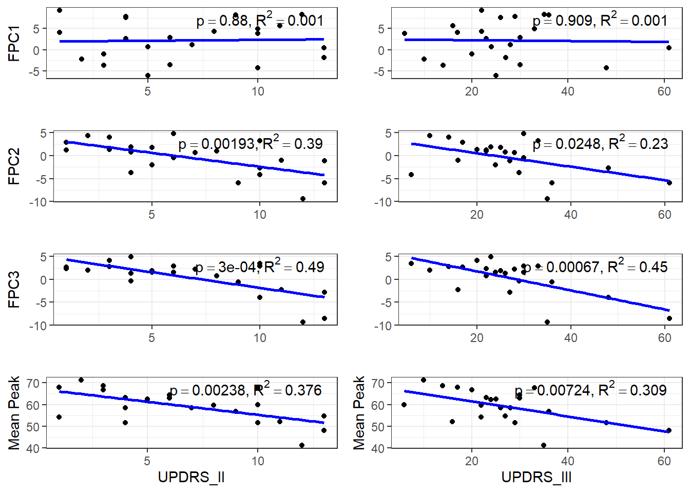
MFPCA projection scores - on/off medication
We now obtain MFPCA projection scores on the “on medication” dataset.
predicted_scores_on = predict_mfpca_scores_wide(
  res_healthy_2way,
  on_dat[,-c(1:3, 104)],
  on_dat$Subject,
  res_healthy_2way$sigma2)

predicted_scores_on = predicted_scores_on %>%
  dplyr::select(ID, L1_PC1, L1_PC2, L1_PC3) %>%
  distinct()
We compute changes compared to the “off medication” scores. We also do this for the clinical MDS-UPDRS scores Part II and Part III, and the mean peak.
change_scores = data.frame(change_FPC1=predicted_scores_on$L1_PC1-predicted_scores_off$L1_PC1,
change_FPC2=predicted_scores_on$L1_PC2-predicted_scores_off$L1_PC2,
change_FPC3=predicted_scores_on$L1_PC3-predicted_scores_off$L1_PC3,
UPDRS_II=as.numeric(diagnosis_wide$UPDRS_II_ON)-as.numeric(diagnosis_wide$UPDRS_II_OFF),
UPDRS_III=as.numeric(diagnosis_wide$UPDRS_II_ON)-as.numeric(diagnosis_wide$UPDRS_III_OFF),
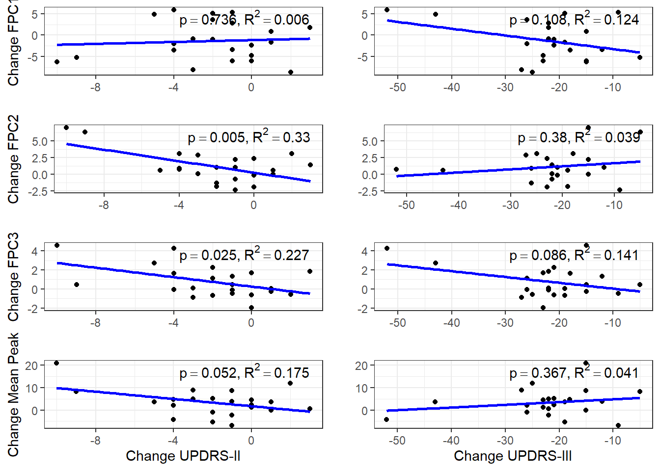
change_peak = peak_data[peak_data$Medication=="on", "mean_peak"]- peak_data[peak_data$Medication=="off", "mean_peak"])We now regress changes in MFPCA projection scores against changes in the clinical outcomes.
change_scores = data.frame(change_FPC1=predicted_scores_on$L1_PC1-predicted_scores_off$L1_PC1,
                           change_FPC2=predicted_scores_on$L1_PC2-predicted_scores_off$L1_PC2,
                           change_FPC3=predicted_scores_on$L1_PC3-predicted_scores_off$L1_PC3,
                     UPDRS_II=as.numeric(diagnosis_wide$UPDRS_II_ON)-as.numeric(diagnosis_wide$UPDRS_II_OFF),
                     UPDRS_III=as.numeric(diagnosis_wide$UPDRS_II_ON)-as.numeric(diagnosis_wide$UPDRS_III_OFF),
                     change_peak = peak_data[peak_data$Medication=="on", "mean_peak"]-  peak_data[peak_data$Medication=="off", "mean_peak"])

summary(lm(change_scores$change_FPC1~change_scores$UPDRS_II))
Call:
lm(formula = change_scores$change_FPC1 ~ change_scores$UPDRS_II)

Residuals:
    Min      1Q  Median      3Q     Max
-7.7978 -3.5626 -0.5697  3.6517  7.4387

Coefficients:
                       Estimate Std. Error t value Pr(>|t|)
(Intercept)             -1.1253     1.1937  -0.943    0.357
change_scores$UPDRS_II   0.1098     0.3217   0.341    0.736

Residual standard error: 4.672 on 20 degrees of freedom
Multiple R-squared:  0.005788,  Adjusted R-squared:  -0.04392
F-statistic: 0.1164 on 1 and 20 DF,  p-value: 0.7365
p1 <- ggplot(change_scores, aes(x=UPDRS_II, y=change_FPC1)) +geom_point() + xlab("")+ylab("Change FPC1")+theme_bw() +
geom_smooth(method = "lm", se = FALSE, color = "blue") +
annotate(
"text",
x = Inf,
y = Inf,
label ="p ==0.736* ',' ~ R^2 == 0.006",
parse = TRUE, hjust = 1.1,
vjust = 1.1
)
summary(lm(change_scores$change_FPC2~change_scores$UPDRS_II))
Call:
lm(formula = change_scores$change_FPC2 ~ change_scores$UPDRS_II)

Residuals:
    Min      1Q  Median      3Q     Max
-3.0656 -1.4493  0.0453  1.4827  3.7519

Coefficients:
                       Estimate Std. Error t value Pr(>|t|)
(Intercept)              0.2359     0.5137   0.459  0.65108
change_scores$UPDRS_II  -0.4334     0.1384  -3.131  0.00526 **
---
Signif. codes:  0 '***' 0.001 '**' 0.01 '*' 0.05 '.' 0.1 ' ' 1

Residual standard error: 2.011 on 20 degrees of freedom
Multiple R-squared:  0.3289,    Adjusted R-squared:  0.2954
F-statistic: 9.803 on 1 and 20 DF,  p-value: 0.005262
p2 <- ggplot(change_scores, aes(x=UPDRS_II, y=change_FPC2)) +geom_point() + xlab("")+ylab("Change FPC2")+theme_bw() +
geom_smooth(method = "lm", se = FALSE, color = "blue") +
annotate(
"text",
x = Inf,
y = Inf,
label ="p ==0.005* ',' ~ R^2 == 0.33",
parse = TRUE,
hjust = 1.1,
vjust = 1.1
)
summary(lm(change_scores$change_FPC3~change_scores$UPDRS_II))
Call:
lm(formula = change_scores$change_FPC3 ~ change_scores$UPDRS_II)

Residuals:
    Min      1Q  Median      3Q     Max
-2.2295 -0.9480 -0.1535  1.1306  2.9971

Coefficients:
                       Estimate Std. Error t value Pr(>|t|)
(Intercept)              0.2704     0.3784   0.715   0.4830
change_scores$UPDRS_II  -0.2468     0.1020  -2.421   0.0251 *
---
Signif. codes:  0 '***' 0.001 '**' 0.01 '*' 0.05 '.' 0.1 ' ' 1

Residual standard error: 1.481 on 20 degrees of freedom
Multiple R-squared:  0.2266,    Adjusted R-squared:  0.188
F-statistic: 5.861 on 1 and 20 DF,  p-value: 0.02512
p3 <- ggplot(change_scores, aes(x=UPDRS_II, y=change_FPC3)) +geom_point() + xlab("")+ylab("Change FPC3")+theme_bw() +
geom_smooth(method = "lm", se = FALSE, color = "blue") +
annotate(
"text",
x = Inf,
y = Inf,
label ="p ==0.025* ',' ~ R^2 == 0.227",
parse = TRUE,
hjust = 1.1,
vjust = 1.1
)
summary(lm(change_scores$mean_peak~change_scores$UPDRS_II))
Call:
lm(formula = change_scores$mean_peak ~ change_scores$UPDRS_II)

Residuals:
    Min      1Q  Median      3Q     Max
-9.4980 -2.7627  0.1493  2.4573 11.7312

Coefficients:
                       Estimate Std. Error t value Pr(>|t|)
(Intercept)              1.7859     1.4570   1.226   0.2345
change_scores$UPDRS_II  -0.8105     0.3926  -2.065   0.0522 .
---
Signif. codes:  0 '***' 0.001 '**' 0.01 '*' 0.05 '.' 0.1 ' ' 1

Residual standard error: 5.702 on 20 degrees of freedom
Multiple R-squared:  0.1757,    Adjusted R-squared:  0.1345
F-statistic: 4.262 on 1 and 20 DF,  p-value: 0.05218
PUII <- ggplot(change_scores, aes(x=UPDRS_II, y=mean_peak)) +geom_point() + xlab("Change UPDRS-II")+ylab("Change Mean Peak")+theme_bw() +
geom_smooth(method = "lm", se = FALSE, color = "blue") +
annotate(
"text",
x = Inf,
y = Inf,
label ="p ==0.052* ',' ~ R^2 == 0.175",
parse = TRUE,
hjust = 1.1,
vjust = 1.1
)
summary(lm(change_scores$change_FPC1~change_scores$UPDRS_III))
Call:
lm(formula = change_scores$change_FPC1 ~ change_scores$UPDRS_III)

Residuals:
    Min      1Q  Median      3Q     Max
-7.8603 -3.0981 -0.1834  3.0197  8.7743

Coefficients:
                        Estimate Std. Error t value Pr(>|t|)
(Intercept)             -4.82261    2.26574  -2.128   0.0459 *
change_scores$UPDRS_III -0.15917    0.09459  -1.683   0.1080
---
Signif. codes:  0 '***' 0.001 '**' 0.01 '*' 0.05 '.' 0.1 ' ' 1

Residual standard error: 4.385 on 20 degrees of freedom
Multiple R-squared:  0.124, Adjusted R-squared:  0.08022
F-statistic: 2.831 on 1 and 20 DF,  p-value: 0.108
p11 <- ggplot(change_scores, aes(x=UPDRS_III, y=change_FPC1)) +geom_point() + xlab("")+ylab("")+theme_bw() +
geom_smooth(method = "lm", se = FALSE, color = "blue") +
annotate(
"text",
x = Inf,
y = Inf,
label ="p ==0.108* ',' ~ R^2 == 0.124",
parse = TRUE,
hjust = 1.1,
vjust = 1.1
)
summary(lm(change_scores$change_FPC2~change_scores$UPDRS_III))
Call:
lm(formula = change_scores$change_FPC2 ~ change_scores$UPDRS_III)

Residuals:
    Min      1Q  Median      3Q     Max
-4.1163 -1.4469 -0.0826  1.2404  5.5399

Coefficients:
                        Estimate Std. Error t value Pr(>|t|)
(Intercept)              2.13957    1.24328   1.721    0.101
change_scores$UPDRS_III  0.04662    0.05191   0.898    0.380

Residual standard error: 2.406 on 20 degrees of freedom
Multiple R-squared:  0.03877,   Adjusted R-squared:  -0.009293
F-statistic: 0.8066 on 1 and 20 DF,  p-value: 0.3798
p22 <- ggplot(change_scores, aes(x=UPDRS_III, y=change_FPC2)) +geom_point() + xlab("")+ylab("")+theme_bw() +
geom_smooth(method = "lm", se = FALSE, color = "blue") +
annotate(
"text",
x = Inf,
y = Inf,
label ="p ==0.380* ',' ~ R^2 == 0.039",
parse = TRUE,
hjust = 1.1,
vjust = 1.1
)
summary(lm(change_scores$change_FPC3~change_scores$UPDRS_III))
Call:
lm(formula = change_scores$change_FPC3 ~ change_scores$UPDRS_III)

Residuals:
    Min      1Q  Median      3Q     Max
-2.8063 -1.0513 -0.1642  1.0010  4.1840

Coefficients:
                        Estimate Std. Error t value Pr(>|t|)
(Intercept)             -0.55308    0.80653  -0.686   0.5007
change_scores$UPDRS_III -0.06088    0.03367  -1.808   0.0856 .
---
Signif. codes:  0 '***' 0.001 '**' 0.01 '*' 0.05 '.' 0.1 ' ' 1

Residual standard error: 1.561 on 20 degrees of freedom
Multiple R-squared:  0.1405,    Adjusted R-squared:  0.09753
F-statistic: 3.269 on 1 and 20 DF,  p-value: 0.08565
p33 <- ggplot(change_scores, aes(x=UPDRS_III, y=change_FPC3)) +geom_point() + xlab("")+ylab("")+theme_bw() +
geom_smooth(method = "lm", se = FALSE, color = "blue") +
annotate(
"text",
x = Inf,
y = Inf,
label ="p ==0.086* ',' ~ R^2 == 0.141",
parse = TRUE,
hjust = 1.1,
vjust = 1.1
)
summary(lm(change_scores$mean_peak~change_scores$UPDRS_III))
Call:
lm(formula = change_scores$mean_peak ~ change_scores$UPDRS_III)

Residuals:
     Min       1Q   Median       3Q      Max
-11.9167  -3.6547  -0.4675   2.4871  16.5964

Coefficients:
                        Estimate Std. Error t value Pr(>|t|)
(Intercept)               6.1184     3.1777   1.925   0.0685 .
change_scores$UPDRS_III   0.1226     0.1327   0.924   0.3665
---
Signif. codes:  0 '***' 0.001 '**' 0.01 '*' 0.05 '.' 0.1 ' ' 1

Residual standard error: 6.15 on 20 degrees of freedom
Multiple R-squared:  0.04094,   Adjusted R-squared:  -0.007009
F-statistic: 0.8538 on 1 and 20 DF,  p-value: 0.3665
PUIII <- ggplot(change_scores, aes(x=UPDRS_III, y=mean_peak)) +geom_point() + xlab("Change UPDRS-III")+ylab("")+theme_bw() +
geom_smooth(method = "lm", se = FALSE, color = "blue") +
annotate(
"text",
x = Inf,
y = Inf,
label ="p ==0.367* ',' ~ R^2 == 0.041",
parse = TRUE,
hjust = 1.1,
vjust = 1.1
)
conv_validity <- ggarrange(
p1,p11,
p2, p22,
p3, p33,
PUII,PUIII,
ncol=2, nrow=4)
conv_validity